Bayesian inference and other things
with the TuringLang ecosystem
Before we begin
Make sure you're in the correct directory
pwd()
"/home/tor/Projects/public/Turing-Workshop/2023-Geilo-Winter-School/Part-2-Turing-and-other-things"
Then run something like (depending on which OS you are on)
julia --project
or if you're already in a REPL, do
]activate .
Activating project at `~/Projects/public/Turing-Workshop/2023-Geilo-Winter-School/Part-2-Turing-and-other-things`
to activate the project
And just to check that you're in the correct one
]status
Project GeiloWinterSchool2023Part2 v0.1.0
Status `~/Projects/public/Turing-Workshop/2023-Geilo-Winter-School/Part-2-Turing-and-other-things/Project.toml`
  [6e4b80f9] BenchmarkTools v1.3.2
  [336ed68f] CSV v0.10.9
  [a93c6f00] DataFrames v1.4.4
⌃ [2b5f629d] DiffEqBase v6.114.1
  [0c46a032] DifferentialEquations v7.6.0
  [31c24e10] Distributions v0.25.80
  [f6369f11] ForwardDiff v0.10.34
  [6fdf6af0] LogDensityProblems v2.1.0
  [996a588d] LogDensityProblemsAD v1.1.1
  [429524aa] Optim v1.7.4
  [c46f51b8] ProfileView v1.5.2
  [37e2e3b7] ReverseDiff v1.14.4 `https://github.com/torfjelde/ReverseDiff.jl#torfjelde/sort-of-support-non-linear-indexing`
  [0bca4576] SciMLBase v1.81.0
⌃ [1ed8b502] SciMLSensitivity v7.17.1
  [f3b207a7] StatsPlots v0.15.4
  [fce5fe82] Turing v0.24.0
  [0db1332d] TuringBenchmarking v0.1.1
  [e88e6eb3] Zygote v0.6.55
Info Packages marked with ⌃ have new versions available and may be upgradable.
Download and install dependencies
]instantiate
And finally, do
using GeiloWinterSchool2023Part2
to get some functionality I've implemented for the occasion
The story of a little Norwegian boy
There once was a little Norwegian boy

When this little boy was 20 years old, he was working as a parking guard near Preikestolen/Pulpit rock

One day it was raining and there was nobody hiking, and so there was no cars in sight for the little boy to point
When his boss wasn't looking, the little 20 year-old boy had an amazing idea
Maybe I can use this method of Mr. Bayes I learned a bit about yesteday to model football / Premier League?
The little boy got very excited and started looking for stuff on the big interwebs
The little boy came across this

And got very excited
But at the time, the little boy knew next to nothing about programming
The little boy couldn't write the code to do the inference
Whence the little boy became a sad little boy :(
But time heals all wounds, and at some point the little boy learned Python
And in Python, the boy found the probabilistic programming language pymc3
Maybe I can use
pymc3to perform inference in that football / Premier League model?
And so the sad boy once more became an excited little boy :)
But there was a problem
The boy wanted to write a for-loop in his model, but the model didn't want it to be so and complained!
The boy got frustrated and gave up, once more becoming a sad little boy :(
The boy should have known that the computational backend theano that was used by pymc3 at the time couldn't handle a for-loop, and instead he should have used scan. But the boy was only 20-something years old; he didn't know.
Some years later the boy discovers a programming language called Julia
Julia makes a few promises
- It's fast. Like really fast.
- It's interactive; doesn't require full compilation for you to play with it.
- You don't have to specify types everywhere.
The boy thinks
Wait, but this sounds like Python but the only difference is that…I CAN WRITE FOR-LOOPS WITHOUT FEELING BAD ABOUT IT?!
Yes, yes he could
And 3.5 years later, he's still writing for-loops. Well, sort of.
Why Turing.jl?
Duh, you should use Turing.jl so you get to use Julia
But even in Julia, other PPLS exist
But Turing.jl is very similar to Julia in "philosophy":
- Flexiblility
- Ease-of-use
- Speed (potentially with a bit of effort)
So it's a pretty good candidate
Running example
We'll work with an outbreak of influenza A (H1N1) in 1978 at a British boarding school
- 763 male students -> 512 of which became ill
- Reported that one infected boy started the epidemic
- Observations are number of boys in bed over 14 days
Data are freely available in the R package outbreaks, maintained as part of the R Epidemics Consortium
Data + part of the analysis is heavily inspired by https://mc-stan.org/users/documentation/case-studies/boarding_school_case_study.html
Stan definitively beats Turing.jl when it comes to great write-ups like these
Loading into Julia
# Load the dataframe.
using Dates
using DataFrames, CSV

N = 763
data = DataFrame(CSV.File(joinpath("data", "influenza_england_1978_school.csv")));
print(data)
14×4 DataFrame
 Row │ Column1  date        in_bed  convalescent
     │ Int64    Date        Int64   Int64
─────┼───────────────────────────────────────────
   1 │       1  1978-01-22       3             0
   2 │       2  1978-01-23       8             0
   3 │       3  1978-01-24      26             0
   4 │       4  1978-01-25      76             0
   5 │       5  1978-01-26     225             9
   6 │       6  1978-01-27     298            17
   7 │       7  1978-01-28     258           105
   8 │       8  1978-01-29     233           162
   9 │       9  1978-01-30     189           176
  10 │      10  1978-01-31     128           166
  11 │      11  1978-02-01      68           150
  12 │      12  1978-02-02      29            85
  13 │      13  1978-02-03      14            47
  14 │      14  1978-02-04       4            20
Notice that each of the columns have associated types
Let's visualize the samples:
using StatsPlots
# StatsPlots.jl provides this convenient macro `@df` for plotting a `DataFrame`.
@df data scatter(:date, :in_bed, label=nothing, ylabel="Number of students in bed")
Differential equations
Suppose we have some function \(f\) which describes how a state \(x\) evolves wrt. \(t\)
which we then need to integrate to obtain the actual state at some time \(t\)
In many interesting scenarios numerical methods are required to obtain \(x(t)\)
In Julia
Everything related to differential equations is provided by DifferentialEquations.jl
And I really do mean everything

Example: SIR model
One particular example of an (ordinary) differential equation that you might have seen recently is the SIR model used in epidemiology

Figure 7: https://covid19.uclaml.org/model.html (2023-01-19)
The temporal dynamics of the sizes of each of the compartments are governed by the following system of ODEs:
where
- \(S(t)\) is the number of people susceptible to becoming infected,
- \(I(t)\) is the number of people currently infected,
- \(R(t)\) is the number of recovered people,
- \(β\) is the constant rate of infectious contact between people,
- \(\gamma\) the constant recovery rate of infected individuals
Converting this ODE into code is just
using DifferentialEquations

function SIR!(
    du,  # buffer for the updated differential equation
    u,   # current state
    p,   # parameters
    t    # current time
)
    N = 763  # population
    S, I, R = u
    β, γ = p

    du[1] = dS = -β * I * S / N
    du[2] = dI = β * I * S / N - γ * I
    du[3] = dR = γ * I
end
SIR! (generic function with 1 method)
Not too bad!
Initial conditions are then
and we want to integrate from \(t = 0\) to \(t = 14\)
# Include 0 because that's the initial condition before any observations.
tspan = (0.0, 14.0)

# Initial conditions are:
#   S(0) = N - 1; I(0) = 1; R(0) = 0
u0 = [N - 1, 1, 0.0]
3-element Vector{Float64}:
 762.0
   1.0
   0.0
Now we just need to define the overall problem and we can solve:
# Just to check that everything works, we'll just use some "totally random" values for β and γ:
problem_sir = let β = 2.0, γ = 0.6
    ODEProblem(SIR!, u0, tspan, (β, γ))
end
ODEProblem with uType Vector{Float64} and tType Float64. In-place: true
timespan: (0.0, 14.0)
u0: 3-element Vector{Float64}:
 762.0
   1.0
   0.0
Aaaand
sol = solve(problem_sir)
retcode: Success
Interpolation: specialized 4th order "free" interpolation, specialized 2nd order "free" stiffness-aware interpolation
t: 23-element Vector{Float64}:
  0.0
  0.0023558376404244326
  0.025914214044668756
  0.11176872871946908
  0.26714420676761075
  0.47653584778586056
  0.7436981238065388
  1.0701182881347182
  1.4556696154809898
  1.8994815718103506
  2.4015425820305163
  2.9657488203418048
  3.6046024613854746
  4.325611232479916
  5.234036476235002
  6.073132270491685
  7.323851265223563
  8.23100744184026
  9.66046960467715
 11.027717843180652
 12.506967592177675
 13.98890399536329
 14.0
u: 23-element Vector{Vector{Float64}}:
 [762.0, 1.0, 0.0]
 [761.9952867607622, 1.003297407481751, 0.001415831756055325]
 [761.9472927630898, 1.036873767352754, 0.015833469557440357]
 [761.7584189579304, 1.1690001128296739, 0.0725809292398516]
 [761.353498610305, 1.4522140137552049, 0.19428737593979384]
 [760.6490369821046, 1.9447820690728455, 0.4061809488225752]
 [759.3950815454128, 2.8210768113583082, 0.7838416432288186]
 [757.0795798160242, 4.437564277195732, 1.4828559067800167]
 [752.6094742865345, 7.552145919430467, 2.8383797940350495]
 [743.573784947305, 13.823077731564027, 5.603137321131049]
 [724.5575481927715, 26.909267078762316, 11.533184728466205]
 [683.6474029897502, 54.51612001957392, 24.836476990675976]
 [598.1841629858786, 109.41164143668018, 55.40419557744127]
 [450.08652743810205, 192.396449154863, 120.51702340703504]
 [259.11626253270623, 256.9925778114915, 246.89115965580237]
 [148.3573731526537, 240.10301213899098, 374.53961470835543]
 [76.52998017846475, 160.6373332952353, 525.8326865263001]
 [55.70519994004921, 108.7634182279299, 598.531381832021]
 [41.39587834423381, 55.09512088924873, 666.5090007665176]
 [35.87067243374374, 27.821838135708532, 699.3074894305479]
 [33.252184333490774, 13.087185981359177, 716.6606296851502]
 [32.08996839417716, 6.105264616193066, 724.8047669896299]
 [32.08428686823946, 6.070415830241046, 724.8452973015196]
We didn't specify a solver
DifferentialEquations.jl uses AutoTsit5(Rosenbrock32()) by default
Which is a composition between
Tsit5(4th order Runge-Kutta), andRosenbrock32(3rd order stiff solver)
with automatic switching between the two
AutoTsit5(Rosenbrock32()) covers many use-cases well, but see
- https://docs.sciml.ai/DiffEqDocs/stable/solvers/ode_solve/
- https://www.stochasticlifestyle.com/comparison-differential-equation-solver-suites-matlab-r-julia-python-c-fortran/
for more info on choosing a solver
This is the resulting solution
plot(
    sol,
    linewidth=2, xaxis="Time in days", label=["Suspectible" "Infected" "Recovered"],
    alpha=0.5, size=(500, 300)
)
scatter!(1:14, data.in_bed, label="Data", color="black")
This doesn't really match the data though; let's do better
Approach #1: find optimal values of \(\beta\) and \(\gamma\) by minimizing some loss, e.g. sum-of-squares
where \(\big( y_i \big)_{i = 1}^{14}\) are the observations, \(F\) is the integrated system
First we define the loss
# Define the loss function.
function loss_sir(problem_orig, p)
    # `remake` just, well, remakes the `problem` with `p` replaced.
    problem = remake(problem_orig, p=p)
    # To ensure we get solutions _exactly_ at the timesteps of interest,
    # i.e. every day we have observations, we use `saveat=1` to tell `solve`
    # to save at every timestep (which is one day).
    sol = solve(problem, saveat=1)
    # Extract the 2nd state, the (I)infected, for the dates with observations.
    sol_for_observed = sol[2, 2:15]
    # Compute the sum-of-squares of the infected vs. data.
    sum(abs2.(sol_for_observed - data.in_bed))
end
loss_sir (generic function with 1 method)
And the go-to for optimization in Julia is Optim.jl
using Optim
# An alternative to writing `y -> f(x, y)` is `Base.Fix1(f, x)` which
# avoids potential performance issues with global variables (as our `problem` here).
opt = optimize(
    p -> loss_sir(problem_sir, p), # function to minimize
    [0, 0],                # lower bounds on variables
    [Inf, Inf],            # upper bounds on variables
    [2.0, 0.5],            # initial values
    Fminbox(NelderMead())  # optimization alg
)
* Status: success

* Candidate solution
   Final objective value:     4.116433e+03

* Found with
   Algorithm:     Fminbox with Nelder-Mead

* Convergence measures
   |x - x'|               = 0.00e+00 ≤ 0.0e+00
   |x - x'|/|x'|          = 0.00e+00 ≤ 0.0e+00
   |f(x) - f(x')|         = 0.00e+00 ≤ 0.0e+00
   |f(x) - f(x')|/|f(x')| = 0.00e+00 ≤ 0.0e+00
   |g(x)|                 = 7.86e+04 ≰ 1.0e-08

* Work counters
   Seconds run:   2  (vs limit Inf)
   Iterations:    4
   f(x) calls:    565
   ∇f(x) calls:   1
We can extract the minimizers of the loss
β, λ = Optim.minimizer(opt)
β, λ
| 1.6692320164955483 | 0.44348639177622445 |
# Solve for the obtained parameters.
problem_sir = remake(problem_sir, p=(β, λ))
sol = solve(problem_sir)

# Plot the solution.
plot(sol, linewidth=2, xaxis="Time in days", label=["Suspectible" "Infected" "Recovered"], alpha=0.5)
# And the data.
scatter!(1:14, data.in_bed, label="Data", color="black")
That's better than our totally "random" guess from earlier!
Example: SEIR model
Adding another compartment to our SIR model: the (E)xposed state
where we've added a new parameter \({\color{orange} \sigma}\) describing the fraction of people who develop observable symptoms in this time
TASK Solve the SEIR model using Julia
function SEIR!(
    du,  # buffer for the updated differential equation
    u,   # current state
    p,   # parameters
    t    # current time
)
    N = 763  # population

    S, E, I, R = u  # have ourselves an additional state!
    β, γ, σ = p     # and an additional parameter!

    # TODO: Implement yah fool!
    du[1] = nothing
    du[2] = nothing
    du[3] = nothing
    du[4] = nothing
end
BONUS: Use Optim.jl to find minimizers of sum-of-squares
SOLUTION Solve the SEIR model using Julia
function SEIR!(
    du,  # buffer for the updated differential equation
    u,   # current state
    p,   # parameters
    t    # current time
)
    N = 763  # population
    S, E, I, R = u  # have ourselves an additional state!
    β, γ, σ = p     # and an additional parameter!

    # Might as well cache these computations.
    βSI = β * S * I / N
    σE = σ * E
    γI = γ * I

    du[1] = -βSI
    du[2] = βSI - σE
    du[3] = σE - γI
    du[4] = γI
end
SEIR! (generic function with 1 method)
problem_seir = let u0 = [N - 1, 0, 1, 0], β = 2.0, γ = 0.6, σ = 0.8
    ODEProblem(SEIR!, u0, tspan, (β, γ, σ))
end
ODEProblem with uType Vector{Int64} and tType Float64. In-place: true
timespan: (0.0, 14.0)
u0: 4-element Vector{Int64}:
 762
   0
   1
   0
sol_seir = solve(problem_seir, saveat=1)
retcode: Success
Interpolation: 1st order linear
t: 15-element Vector{Float64}:
  0.0
  1.0
  2.0
  3.0
  4.0
  5.0
  6.0
  7.0
  8.0
  9.0
 10.0
 11.0
 12.0
 13.0
 14.0
u: 15-element Vector{Vector{Float64}}:
 [762.0, 0.0, 1.0, 0.0]
 [760.1497035901518, 1.277915971753478, 1.0158871356490553, 0.5564933024456415]
 [757.5476928906271, 2.425869618233348, 1.6850698824327135, 1.341367608706787]
 [753.081189706403, 4.277014534677882, 2.9468385687120784, 2.6949571902067637]
 [745.3234082630842, 7.455598293492679, 5.155811621098981, 5.065181822323938]
 [731.9851682751213, 12.855816151849933, 8.960337047554939, 9.198678525473571]
 [709.5042941973462, 21.77178343781762, 15.384985521594787, 16.338936843241182]
 [672.8733895183619, 35.77263271085456, 25.88133104438007, 28.472646726403138]
 [616.390571176038, 55.97177756967422, 42.09614416178476, 48.54150709250279]
 [536.453596476594, 81.2428045994271, 64.9673325777641, 80.33626634621449]
 [436.43708330634297, 106.04037246704702, 92.9550757379631, 127.56746848864664]
 [329.60092931771436, 121.08020372279418, 120.48402926084937, 191.83483769864185]
 [233.8471941518982, 119.43669383157659, 139.3233304893263, 270.3927815271987]
 [160.88805352426687, 102.7399386960996, 143.3826208089892, 355.9893869706441]
 [111.72261866282292, 79.02493776169311, 132.78384886713565, 439.46859470834806]
plot(sol_seir, linewidth=2, xaxis="Time in days", label=["Suspectible" "Exposed" "Infected" "Recovered"], alpha=0.5)
scatter!(1:14, data.in_bed, label="Data")
Don't look so good. Let's try Optim.jl again.
function loss_seir(problem, p)
    problem = remake(problem, p=p)
    sol = solve(problem, saveat=1)
    # NOTE: 3rd state is now the (I)nfectious compartment!!!
    sol_for_observed = sol[3, 2:15]
    return sum(abs2.(sol_for_observed - data.in_bed))
end
loss_seir (generic function with 1 method)
opt = optimize(Base.Fix1(loss_seir, problem_seir), [0, 0, 0], [Inf, Inf, Inf], [2.0, 0.5, 0.9], Fminbox(NelderMead()))
* Status: success (reached maximum number of iterations)

* Candidate solution
   Final objective value:     3.115978e+03

* Found with
   Algorithm:     Fminbox with Nelder-Mead

* Convergence measures
   |x - x'|               = 0.00e+00 ≤ 0.0e+00
   |x - x'|/|x'|          = 0.00e+00 ≤ 0.0e+00
   |f(x) - f(x')|         = 0.00e+00 ≤ 0.0e+00
   |f(x) - f(x')|/|f(x')| = 0.00e+00 ≤ 0.0e+00
   |g(x)|                 = 1.77e+05 ≰ 1.0e-08

* Work counters
   Seconds run:   1  (vs limit Inf)
   Iterations:    3
   f(x) calls:    13259
   ∇f(x) calls:   1
β, γ, σ = Optim.minimizer(opt)
3-element Vector{Float64}:
 4.853872993924619
 0.4671485850111774
 0.8150294098438762
sol_seir = solve(remake(problem_seir, p=(β, γ, σ)), saveat=1)
plot(sol_seir, linewidth=2, xaxis="Time in days", label=["Suspectible" "Exposed" "Infected" "Recovered"], alpha=0.5)
scatter!(1:14, data.in_bed, label="Data", color="black")
But…but these are point estimates! What about distributions? WHAT ABOUT UNCERTAINTY?!
No, no that's fair.
Let's do some Bayesian inference then.
BUT FIRST!
Making our future selves less annoyed
It's annoying to have all these different loss-functions for both SIR! and SEIR!
# Abstract type which we can use to dispatch on.
abstract type AbstractEpidemicProblem end

struct SIRProblem{P} <: AbstractEpidemicProblem
    problem::P
    N::Int
end

function SIRProblem(N::Int; u0 = [N - 1, 1, 0.], tspan = (0, 14), p = [2.0, 0.6])
    return SIRProblem(ODEProblem(SIR!, u0, tspan, p), N)
end
SIRProblem
Then we can just construct the problem as
sir = SIRProblem(N);
And to make it a bit easier to work with, we add some utility functions
# General.
parameters(prob::AbstractEpidemicProblem) = prob.problem.p
initial_state(prob::AbstractEpidemicProblem) = prob.problem.u0
population(prob::AbstractEpidemicProblem) = prob.N

# Specializations.
susceptible(::SIRProblem, u::AbstractMatrix) = u[1, :]
infected(::SIRProblem, u::AbstractMatrix) = u[2, :]
recovered(::SIRProblem, u::AbstractMatrix) = u[3, :]
recovered (generic function with 2 methods)
So that once we've solved the problem, we can easily extract the compartment we want, e.g.
sol = solve(sir.problem, saveat=1)
infected(sir, sol)
15-element Vector{Float64}:
   1.0
   4.026799533924021
  15.824575905720002
  56.779007685250534
 154.4310579906169
 248.98982384839158
 243.67838619968524
 181.93939659551987
 120.64627375763271
  75.92085282572398
  46.58644927641269
  28.214678599716418
  16.96318676577873
  10.158687874394722
   6.070415830241046
TASK Implement SEIRProblem
struct SEIRProblem <: AbstractEpidemicProblem
    # ...
end

function SEIRProblem end

susceptible
exposed
infected
recovered
SOLUTION Implement SEIRProblem
struct SEIRProblem{P} <: AbstractEpidemicProblem
    problem::P
    N::Int
end

function SEIRProblem(N::Int; u0 = [N - 1, 0, 1, 0.], tspan = (0, 14), p = [4.5, 0.45, 0.8])
    return SEIRProblem(ODEProblem(SEIR!, u0, tspan, p), N)
end

susceptible(::SEIRProblem, u::AbstractMatrix) = u[1, :]
exposed(::SEIRProblem, u::AbstractMatrix) = u[2, :]
infected(::SEIRProblem, u::AbstractMatrix) = u[3, :]
recovered(::SEIRProblem, u::AbstractMatrix) = u[4, :]
recovered (generic function with 2 methods)
Now, given a problem and a sol, we can query the sol for the infected state without explicit handling of which problem we're working with
seir = SEIRProblem(N);
sol = solve(seir.problem, saveat=1)
infected(seir, sol)
15-element Vector{Float64}:
   1.0
   1.9941817088874336
   6.958582307202902
  23.9262335176065
  74.23638542794971
 176.98368495653585
 276.06126059898344
 293.92632518571605
 249.92836195453708
 189.07578975511504
 134.2373192679034
  91.82578430804273
  61.38108478932363
  40.42264366743211
  26.357816296754425
Same loss for both!
function loss(problem_wrapper::AbstractEpidemicProblem, p)
    # NOTE: Extract the `problem` from `problem_wrapper`.
    problem = remake(problem_wrapper.problem, p=p)
    sol = solve(problem, saveat=1)
    # NOTE: Now this is completely general!
    sol_for_observed = infected(problem_wrapper, sol)[2:end]
    return sum(abs2.(sol_for_observed - data.in_bed))
end
loss (generic function with 1 method)
Now we can call the same loss for both SIR and SEIR
loss(SIRProblem(N), [2.0, 0.6])
50257.83978134881
loss(SEIRProblem(N), [2.0, 0.6, 0.8])
287325.105532706
Bayesian inference
First off
using Turing
This dataset really doesn't have too many observations
nrow(data)
14
So reporting a single number for parameters is maybe being a bit too confident
We'll use the following model
where
- \(\big( y_i \big)_{i = 1}^{14}\) are the observations,
- \(F\) is the integrated system, and
- \(\phi\) is the over-dispersion parameter.
plot(
    plot(truncated(Normal(2, 1); lower=0), label=nothing, title="β"),
    plot(truncated(Normal(0.4, 0.5); lower=0), label=nothing, title="γ"),
    plot(Exponential(1/5), label=nothing, title="ϕ⁻¹"),
    layout=(3, 1)
)

A NegativeBinomial(r, p) represents the number of trials to achieve \(r\) successes, where each trial has a probability \(p\) of success
A NegativeBinomial2(μ, ϕ) is the same, but parameterized using the mean \(μ\) and dispersion \(\phi\)
# `NegativeBinomial` already exists, so let's just make an alternative constructor instead.
function NegativeBinomial2(μ, ϕ)
    p = 1/(1 + μ/ϕ)
    r = ϕ
    return NegativeBinomial(r, p)
end
NegativeBinomial2 (generic function with 1 method)
# Let's just make sure we didn't do something stupid.
μ = 2; ϕ = 3;
dist = NegativeBinomial2(μ, ϕ)
# Source: https://mc-stan.org/docs/2_20/functions-reference/nbalt.html
mean(dist) ≈ μ && var(dist) ≈ μ + μ^2 / ϕ
true
Can be considered a generalization of Poisson
μ = 2.0
anim = @animate for ϕ ∈ [0.1, 0.5, 1.0, 2.0, 5.0, 10.0, 25.0, 100.0]
    p = plot(size=(500, 300))
    plot!(p, Poisson(μ); label="Poisson($μ)")
    plot!(p, NegativeBinomial2(μ, ϕ), label="NegativeBinomial2($μ, $ϕ)")
    xlims!(0, 20); ylims!(0, 0.35);
    p
end
gif(anim, "negative_binomial.gif", fps=2);
[ Info: Saved animation to /home/tor/Projects/public/Turing-Workshop/2023-Geilo-Winter-School/Part-2-Turing-and-other-things/negative_binomial.gif
@model function sir_model(
    num_days;                                  # Number of days to model
    tspan = (0.0, float(num_days)),            # Timespan to model
    u0 = [N - 1, 1, 0.0],                      # Initial state
    p0 = [2.0, 0.6],                           # Placeholder parameters
    problem = ODEProblem(SIR!, u0, tspan, p0)  # Create problem once so we can `remake`.
)
    β ~ truncated(Normal(2, 1); lower=0)
    γ ~ truncated(Normal(0.4, 0.5); lower=0)
    ϕ⁻¹ ~ Exponential(1/5)
    ϕ = inv(ϕ⁻¹)

    problem_new = remake(problem, p=[β, γ])  # Replace parameters `p`.
    sol = solve(problem_new, saveat=1)       # Solve!

    sol_for_observed = sol[2, 2:num_days + 1]  # Timesteps we have observations for.
    in_bed = Vector{Int}(undef, num_days)
    for i = 1:length(sol_for_observed)
        # Add a small constant to `sol_for_observed` to make things more stable.
        in_bed[i] ~ NegativeBinomial2(sol_for_observed[i] + 1e-5, ϕ)
    end

    # Some quantities we might be interested in.
    return (R0 = β / γ, recovery_time = 1 / γ, infected = sol_for_observed)
end
sir_model (generic function with 2 methods)
Let's break it down
β ~ truncated(Normal(2, 1); lower=0)
γ ~ truncated(Normal(0.4, 0.5); lower=0)
ϕ⁻¹ ~ Exponential(1/5)
ϕ = inv(ϕ⁻¹)
defines our prior
truncated is just a way of restricting the domain of the distribution you pass it
problem_new = remake(problem, p=[β, γ])  # Replace parameters `p`.
sol = solve(problem_new, saveat=1)       # Solve!
We then remake the problem, now with the parameters [β, γ] sampled above
saveat = 1 gets us the solution at the timesteps [0, 1, 2, ..., 14]
Then we extract the timesteps we have observations for
sol_for_observed = sol[2, 2:num_days + 1] # Timesteps we have observations for.
and define what's going to be a likelihood (once we add observations)
in_bed = Vector{Int}(undef, num_days)
for i = 1:length(sol_for_observed)
    # Add a small constant to `sol_for_observed` to make things more stable.
    in_bed[i] ~ NegativeBinomial2(sol_for_observed[i] + 1e-5, ϕ)
end
Finally we return some values that might be of interest to
# Some quantities we might be interested in.
return (R0 = β / γ, recovery_time = 1 / γ, infected = sol_for_observed)
This is useful for a post-sampling diagnostics, debugging, etc.
model = sir_model(length(data.in_bed))
Model(
  args = (:num_days, :tspan, :u0, :p0, :problem)
  defaults = (:tspan, :u0, :p0, :problem)
  context = DynamicPPL.DefaultContext()
)
The model is just another function, so we can call it to check that it works
model().infected
14-element Vector{Float64}:
   4.629880098761509
  20.51149899075346
  76.01682025343723
 170.19683994223317
 188.1484617193551
 130.8534765547809
  74.41578155120635
  38.968883878630315
  19.70373448216648
   9.79913321292256
   4.837363010506036
   2.3788515858966703
   1.167609404493511
   0.5726457769454385
Hey, it does!
Is the prior reasonable?
Before we do any inference, we should check if the prior is reasonable
From domain knowledge we know that (for influenza at least)
- \(R_0\) is typically between 1 and 2
recovery_time(\(1 / \gamma\)) is usually ~1 week
We want to make sure that your prior belief reflects this knowledge while still being flexible enough to accommodate the observations
To check this we'll just simulate some draws from our prior model, i.e. the model without conditioning on in_bed
There are two ways to sample form the prior
# 1. By just calling the `model`, which returns a `NamedTuple` containing the quantities of interest
print(model())
(R0 = 1.5744220262579935, recovery_time = 1.0914322040400142, infected = [1.686706278885068, 2.8316832197830895, 4.716863573067216, 7.756274929408289, 12.489841589345032, 19.460362335608362, 28.856011572547263, 39.90424926578871, 50.43351515502132, 57.45932083686618, 58.82922439267481, 54.59403067743465, 46.666918039077295, 37.41622088550463])
Or by just calling sample using Prior
# Sample from prior.
chain_prior = sample(model, Prior(), 10_000);
Sampling:  17%|███████                                  |  ETA: 0:00:01
Sampling:  38%|███████████████▋                         |  ETA: 0:00:01
Sampling:  58%|███████████████████████▋                 |  ETA: 0:00:00
Sampling:  72%|█████████████████████████████▊           |  ETA: 0:00:00
Sampling:  87%|███████████████████████████████████▋     |  ETA: 0:00:00
Sampling: 100%|█████████████████████████████████████████| Time: 0:00:00
Let's have a look at the prior predictive
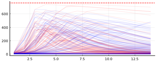
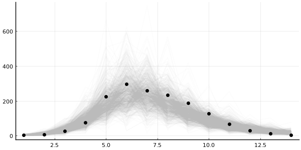
p = plot(legend=false, size=(600, 300))
plot_trajectories!(p, group(chain_prior, :in_bed); n = 1000)
hline!([N], color="red")
For certain values we get number of infected larger than the actual population
But this is includes the randomness from NegativeBinomial2 likelihood
Maybe more useful to inspect the (I)nfected state from the ODE solution?
We can also look at the generated_quantities, i.e. the values from the return statement in our model
Our return looked like this
# Some quantities we might be interested in.
return (R0 = β / γ, recovery_time = 1 / γ, infected = sol_for_observed)
and so generated_quantities (conditioned on chain_prior) gives us
quantities_prior = generated_quantities(
    model,
    MCMCChains.get_sections(chain_prior, :parameters)
)
print(quantities_prior[1])
(R0 = 4.605690136988736, recovery_time = 2.233647692485423, infected = [4.984997209753707, 24.029092981830093, 99.82240918848625, 261.07361336182714, 344.54043982014423, 295.98314301752475, 215.79118631762378, 148.29201252405755, 99.44804435344652, 65.92385902526553, 43.43722911865047, 28.520552363047532, 18.69045660211042, 12.232600393221547])
We can convert it into a Chains using a utility function of mine
# Convert to `Chains`.
chain_quantities_prior = to_chains(quantities_prior);
# Plot.
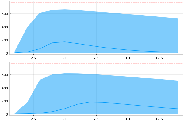
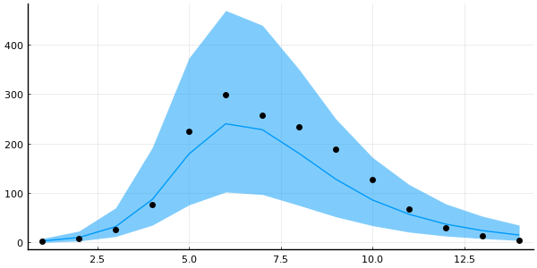
p = plot(legend=false, size=(600, 300))
plot_trajectories!(p, group(chain_quantities_prior, :infected); n = 1000)
hline!([N], color="red")
NOTE: to_chains is not part of "official" Turing.jl because the return can contain whatever you want, and so it's not always possible to convert into a Chains
And the quantiles for the trajectories
p = plot(legend=false, size=(600, 300))
plot_trajectory_quantiles!(p, group(chain_quantities_prior, :infected))
hline!(p, [N], color="red")
DataFrame(quantile(chain_quantities_prior[:, [:R0, :recovery_time], :]))
2×6 DataFrame
 Row │ parameters     2.5%      25.0%    50.0%    75.0%    97.5%
     │ Symbol         Float64   Float64  Float64  Float64  Float64
─────┼─────────────────────────────────────────────────────────────
   1 │ R0             0.487053  2.09801  3.70619  7.31515  62.3576
   2 │ recovery_time  0.706025  1.21271  1.88363  3.46962  29.1143
Compare to our prior knowledge of \(R_0 \in [1, 2]\) and \((1/\gamma) \approx 1\) for influenza
Do we really need probability mass on \(R_0 \ge 10\)?
TASK What's wrong with the current prior?
The SIR model
And here's the current priors
plot(
    plot(truncated(Normal(2, 1); lower=0), label=nothing, title="β"),
    plot(truncated(Normal(0.4, 0.5); lower=0), label=nothing, title="γ"),
    plot(Exponential(1/5), label=nothing, title="ϕ⁻¹"),
    layout=(3, 1)
)
SOLUTION Recovery time shouldn't be several years
We mentioned that recovery_time, which is expressed as \(1 / \gamma\), is ~1 week
We're clearly putting high probability on regions near 0, i.e. long recovery times
plot(truncated(Normal(0.4, 0.5); lower=0), label=nothing, title="γ", size=(500, 300))
Should probably be putting less probability mass near 0
SOLUTION \({\color{red} \gamma}\) should not be larger than 1
If \({\color{red} \gamma} > 1\) ⟹ (R)ecovered increase by more than the (I)nfected
⟹ healthy people are recovering
This was, rightly so, contested when I presented this, as the conservation is preserved by the system independent of the value of \(\gamma\) (as long as it's positive). There is an argument to be made about having a recovery time of <1 day, i.e. \(\gamma > 1\), being unreasonable, but the reasoning above is incorrect!
Just to convince ourselves that it is indeed not a problem with \(\gamma > 1\), we can just run the model with a large \(\gamma\) and look at the in_bed under this prior.
model_gamma = model | (γ = 1.5, )
chain_gamma = sample(model_gamma, Prior(), 10_000, progress=false)

p1 = plot_trajectories!(plot(legend=false), group(chain_gamma, :in_bed))
hline!(p1, [N], color="red")

p2 = plot_trajectory_quantiles!(plot(legend=false), group(chain_gamma, :in_bed))
hline!(p2, [N], color="red")

plot(p1, p2, layout=(2,1), size=(600, 400))
Maybe something like
plot(Beta(2, 5), label="new", size=(500, 300))
plot!(truncated(Normal(0.4, 0.5); lower=0), label="old", color="red")
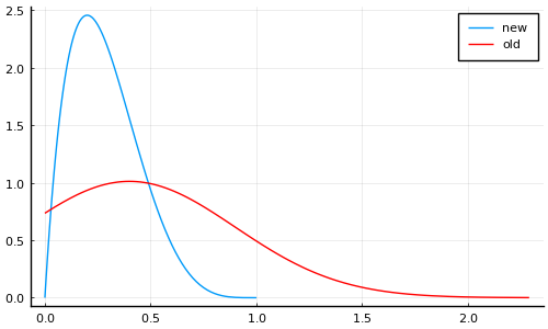
[X]Bounded at 1 to exlcude recovery time of less than 1 day[X]Allows smaller values (i.e. longer recovery time) but rapidly decreases near zero
SOLUTION What if \({\color{red} \beta} > N\)?
Then for \(t = 0\) we have
i.e. we immediately infect everyone on the very first time-step
Also doesn't seem very realistic
But under our current prior does this matter?
# ℙ(β > N) = 1 - ℙ(β ≤ N)
1 - cdf(truncated(Normal(2, 1); lower=0), N)
0.0
Better yet
quantile(truncated(Normal(2, 1); lower=0), 0.95)
3.6559843567138275
i.e. 95% of the probability mass falls below ~3.65
⟹ Current prior for \(\beta\) seems fine (✓)
Before we change the prior, let's also make it a bit easier to change the prior using @submodel
@submodel allows you call models within models, e.g.
@model function A()
    x_hidden_from_B ~ Normal()
    x = x_hidden_from_B + 100
    return x
end

@model function B()
    @submodel x = A()
    y ~ Normal(x, 1)

    return (; x, y)
end
B (generic function with 2 methods)
# So if we call `B` we only see `x` and `y`
println(B()())
(x = 101.54969461293537, y = 102.48444715535948)
# While if we sample from `B` we get the latent variables
println(rand(B()))
(x_hidden_from_B = 0.18899969500711336, y = 99.3704062023967)
To avoid clashes of variable-names, we can specify a prefix
@model A() = (x ~ Normal(); return x + 100)

@model function B()
    # Given it a prefix to use for the variables in `A`.
    @submodel prefix=:inner x_inner = A()
    x ~ Normal(x_inner, 1)

    return (; x_inner, x)
end
B (generic function with 2 methods)
print(rand(B()))
(var"inner.x" = 0.45580772395367214, x = 100.5643900955249)
@submodel is useful as it allows you to:
- Easy to swap out certain parts of your model.
- Can re-use models across projects and packages.
When working on larger projects, this really shines
Equipped with @submodel we can replace
β ~ truncated(Normal(2, 1); lower=0)
γ ~ truncated(Normal(0.4, 0.5); lower=0)
with
@submodel p = prior(problem_wrapper)
where prior can be something like
@model function prior_original(problem_wrapper::SIRProblem)
    β ~ truncated(Normal(2, 1); lower=0)
    γ ~ truncated(Normal(0.4, 0.5); lower=0)

    return [β, γ]
end

@model function prior_improved(problem_wrapper::SIRProblem)
    # NOTE: Should probably also lower mean for `β` since
    # more probability mass on small `γ` ⟹ `R0 =  β / γ` grows.
    β ~ truncated(Normal(1, 1); lower=0)
    # NOTE: New prior for `γ`.
    γ ~ Beta(2, 5)

    return [β, γ]
end
prior_improved (generic function with 2 methods)
@model function epidemic_model(
    problem_wrapper::AbstractEpidemicProblem,
    prior  # NOTE: now we just pass the prior as an argument
)
    # NOTE: And use `@submodel` to embed the `prior` in our model.
    @submodel p = prior(problem_wrapper)

    ϕ⁻¹ ~ Exponential(1/5)
    ϕ = inv(ϕ⁻¹)

    problem_new = remake(problem_wrapper.problem, p=p)  # Replace parameters `p`.
    sol = solve(problem_new, saveat=1)                  # Solve!

    # Extract the `infected`.
    sol_for_observed = infected(problem_wrapper, sol)[2:end]

    # NOTE: `arraydist` is faster for larger dimensional problems,
    # and it does not require explicit allocation of the vector.
    in_bed ~ arraydist(NegativeBinomial2.(sol_for_observed .+ 1e-5, ϕ))

    β, γ = p[1:2]
    return (R0 = β / γ, recovery_time = 1 / γ, infected = sol_for_observed)
end
epidemic_model (generic function with 3 methods)
Another neat trick is to return early if integration fail
@model function epidemic_model(
    problem_wrapper::AbstractEpidemicProblem,
    prior  # now we just pass the prior as an argument
)
    # And use `@submodel` to embed the `prior` in our model.
    @submodel p = prior(problem_wrapper)

    ϕ⁻¹ ~ Exponential(1/5)
    ϕ = inv(ϕ⁻¹)

    problem_new = remake(problem_wrapper.problem, p=p)  # Replace parameters `p`.
    sol = solve(problem_new, saveat=1)                  # Solve!

    # NOTE: Return early if integration failed.
    if !issuccess(sol)
        Turing.@addlogprob! -Inf  # NOTE: Causes automatic rejection.
        return nothing
    end

    # Extract the `infected`.
    sol_for_observed = infected(problem_wrapper, sol)[2:end]

    # `arraydist` is faster for larger dimensional problems,
    # and it does not require explicit allocation of the vector.
    in_bed ~ arraydist(NegativeBinomial2.(sol_for_observed .+ 1e-5, ϕ))

    β, γ = p[1:2]
    return (R0 = β / γ, recovery_time = 1 / γ, infected = sol_for_observed)
end
epidemic_model (generic function with 3 methods)
Equipped with this we can now easily construct two models using different priors
sir = SIRProblem(N);
model_original = epidemic_model(sir, prior_original);
model_improved = epidemic_model(sir, prior_improved);
but using the same underlying epidemic_model
chain_prior_original = sample(model_original, Prior(), 10_000; progress=false);
chain_prior_improved = sample(model_improved, Prior(), 10_000; progress=false);
Let's compare the resulting priors over some of the quantities of interest
Let's compare the generated_quantities, e.g. \(R_0\)
chain_quantities_original = to_chains(
    generated_quantities(
        model_original,
        MCMCChains.get_sections(chain_prior_original, :parameters)
    );
);

chain_quantities_improved = to_chains(
    generated_quantities(
        model_improved,
        MCMCChains.get_sections(chain_prior_improved, :parameters)
    );
);
p = plot(; legend=false, size=(500, 200))
plot_trajectories!(p, group(chain_quantities_original, :infected); n = 100, trajectory_color="red")
plot_trajectories!(p, group(chain_quantities_improved, :infected); n = 100, trajectory_color="blue")
hline!([N], color="red", linestyle=:dash)
plt1 = plot(legend=false)
plot_trajectory_quantiles!(plt1, group(chain_quantities_original, :infected))
hline!(plt1, [N], color="red", linestyle=:dash)

plt2 = plot(legend=false)
plot_trajectory_quantiles!(plt2, group(chain_quantities_improved, :infected))
hline!(plt2, [N], color="red", linestyle=:dash)

plot(plt1, plt2, layout=(2, 1))
This makes sense: if half of the population is immediately infected ⟹ number of infected tapers wrt. time as they recover
For model_improved we then have
DataFrame(quantile(chain_quantities_improved[:, [:R0, :recovery_time], :]))
2×6 DataFrame
 Row │ parameters     2.5%      25.0%    50.0%    75.0%    97.5%
     │ Symbol         Float64   Float64  Float64  Float64  Float64
─────┼─────────────────────────────────────────────────────────────
   1 │ R0             0.295478  2.30191  4.52993  8.41333  35.9603
   2 │ recovery_time  1.55995   2.55853  3.81049  6.31316  23.6136
Compare to model_original
DataFrame(quantile(chain_quantities_original[:, [:R0, :recovery_time], :]))
2×6 DataFrame
 Row │ parameters     2.5%      25.0%    50.0%    75.0%    97.5%
     │ Symbol         Float64   Float64  Float64  Float64  Float64
─────┼─────────────────────────────────────────────────────────────
   1 │ R0             0.495283  2.10977  3.7219   7.30474  59.9345
   2 │ recovery_time  0.693234  1.20832  1.88465  3.48181  29.4579
TASK Make epidemic_model work for SEIRProblem
[ ]Implement a prior which also includes \(\sigma\) and executeepidemic_modelwith it[ ]Can we make a better prior for \(\sigma\)? Do we even need one?
@model function prior_original(problem_wrapper::SEIRProblem)
    # TODO: Implement
end
SOLUTION
@model function prior_original(problem_wrapper::SEIRProblem)
    β ~ truncated(Normal(2, 1); lower=0)
    γ ~ truncated(Normal(0.4, 0.5); lower=0)
    σ ~ truncated(Normal(0.8, 0.5); lower=0)

    return [β, γ, σ]
end
prior_original (generic function with 4 methods)
model_seir = epidemic_model(SEIRProblem(N), prior_original)
print(model_seir())
(R0 = 1.249905922185047, recovery_time = 1.1275375476185503, infected = [0.41458760197101757, 0.175982147386383, 0.07874256170480576, 0.03911764946193381, 0.02298161307777028, 0.01641950959805482, 0.013759122196211936, 0.012689081710378131, 0.012267493170560804, 0.012110652999146742, 0.012061533724674748, 0.012055660061838289, 0.01206858103422115, 0.012088341860835633])
WARNING Consult with domain experts
This guy should not be the one setting your priors!
Get an actual scientist to do that…
Condition
Now let's actually involve the data
We can condition a Model as so
# Condition on the observations.
model = epidemic_model(SIRProblem(N), prior_improved)
model_conditioned = model | (in_bed = data.in_bed,)
Model(
  args = (:problem_wrapper, :prior)
  defaults = ()
  context = ConditionContext((in_bed = [3, 8, 26, 76, 225, 298, 258, 233, 189, 128, 68, 29, 14, 4],), DynamicPPL.DefaultContext())
)
You know what time it is: inference time!
Metropolis-Hastings (MH)
chain_mh = sample(model_conditioned, MH(), MCMCThreads(), 10_000, 4; discard_initial=5_000);
Rhat is okay-ish but not great, and ESS is pretty low innit?
plot(chain_mh; size=(800, 500))
Eeehh doesn't look the greatest
Difficult to trust these results, but let's check if it at least did something useful
# We're using the unconditioned model!
predictions_mh = predict(model, chain_mh)
Chains MCMC chain (10000×14×4 Array{Float64, 3}):

Iterations        = 1:1:10000
Number of chains  = 4
Samples per chain = 10000
parameters        = in_bed[1], in_bed[2], in_bed[3], in_bed[4], in_bed[5], in_bed[6], in_bed[7], in_bed[8], in_bed[9], in_bed[10], in_bed[11], in_bed[12], in_bed[13], in_bed[14]
internals         =

Summary Statistics
  parameters       mean       std   naive_se      mcse          ess      rhat
      Symbol    Float64   Float64    Float64   Float64      Float64   Float64

   in_bed[1]     3.3239    2.1843     0.0109    0.0157   30552.3306    1.0007
   in_bed[2]    10.9294    5.2800     0.0264    0.0765    3416.2516    1.0035
   in_bed[3]    34.2420   15.1777     0.0759    0.3451    1224.2460    1.0094
   in_bed[4]    93.9719   40.8019     0.2040    1.0230     986.9341    1.0117
   in_bed[5]   189.9567   76.0954     0.3805    1.6855    1228.9914    1.0092
   in_bed[6]   251.4305   93.8553     0.4693    1.3148    3319.4564    1.0035
   in_bed[7]   238.4202   87.8089     0.4390    1.0119    5807.9491    1.0019
   in_bed[8]   187.8321   70.0577     0.3503    1.0287    3162.2209    1.0030
   in_bed[9]   133.3270   50.5663     0.2528    0.8771    2085.0535    1.0031
  in_bed[10]    90.4691   35.6730     0.1784    0.6878    1522.7552    1.0053
  in_bed[11]    60.0969   24.7118     0.1236    0.5338    1282.4864    1.0065
  in_bed[12]    39.1181   16.8669     0.0843    0.3941    1036.7038    1.0085
  in_bed[13]    25.4850   11.6236     0.0581    0.2900     899.2603    1.0112
  in_bed[14]    16.4625    8.0545     0.0403    0.2026     874.3031    1.0101

Quantiles
  parameters       2.5%      25.0%      50.0%      75.0%      97.5%
      Symbol    Float64    Float64    Float64    Float64    Float64

   in_bed[1]     0.0000     2.0000     3.0000     5.0000     8.0000
   in_bed[2]     3.0000     7.0000    10.0000    14.0000    23.0000
   in_bed[3]    12.0000    24.0000    32.0000    42.0000    70.0000
   in_bed[4]    35.0000    67.0000    87.0000   113.0000   192.0000
   in_bed[5]    76.0000   138.0000   179.0000   228.0000   373.0000
   in_bed[6]   102.0000   188.0000   240.0000   301.0000   469.0000
   in_bed[7]    97.0000   178.0000   228.0000   287.0000   439.0000
   in_bed[8]    75.0000   140.0000   180.0000   226.0000   350.0000
   in_bed[9]    52.0000    98.0000   128.0000   161.0000   250.0000
  in_bed[10]    34.0000    66.0000    86.0000   110.0000   172.0000
  in_bed[11]    21.0000    43.0000    57.0000    73.0000   117.0000
  in_bed[12]    13.0000    28.0000    37.0000    48.0000    78.0000
  in_bed[13]     8.0000    17.0000    24.0000    32.0000    53.0000
  in_bed[14]     4.0000    11.0000    15.0000    21.0000    35.0000
plot_trajectories!(plot(legend=false, size=(600, 300)), predictions_mh; data=data)
plot_trajectory_quantiles!(plot(legend=false, size=(600, 300)), predictions_mh; data=data)
Okay, it's not completely useless, but my trust-issues are still present.
Metropolis-Hastings have disappointed me one too many times before.
So instead, let's go NUTS
That's right, we're reaching to the No U-Turn sampler (NUTS)
Wooaah there!
NUTSrequires gradient information!How are you going to get that through that
solve?
Good question, voice in my head
I'm obviously not going to it myself
Automatic differentiation (AD) in Julia
- ForwardDiff.jl: forward-mode AD (default in Turing.jl)
- ReverseDiff.jl: tape-based reverse-mode AD
- Zygote.jl: source-to-source reverse-mode AD
- And more…
Up-and-coming
- Enzyme.jl: Julia bindings for Enzyme which ADs LLVM (low-level)
- Diffractor.jl: experimental mixed-mode AD meant to replace Zygote.jl
Of importance
- ChainRulesCore.jl: light-weight package for defining rules, compatible with many of the above
Important
When you write code, you don't have to make a choice which one you want to use!
All the (stable) ones, will (mostly) work
But how you write code will affect performance characteristics
Takes a bit of know-how + a bit of digging to go properly "vroom!"
Differentiating through solve
With that being said, differentiating through numerical solve is not necessarily trivial to do efficiently
There are numerous ways of approaching this problem

https://arxiv.org/abs/1812.01892 is great resource
But this is why we have SciMLSensitivity.jl
SciMLSensitivity.jl docs also provides a great overview of different approaches
using SciMLSensitivity
It offers
- Discrete sensitivity analysis or the "Direct" method: just use
ForwardDiff.Dualin thesolve. - Continuous local sensitivity analysis (CSA): extends the original
system such that the
solvegives you both the solution and the the gradient simultaenously. - Adjoint methods: construct a backwards system whose solution gives us the gradient.
Just do solve(problem, solver, sensealg = ...)
Back to being NUTS
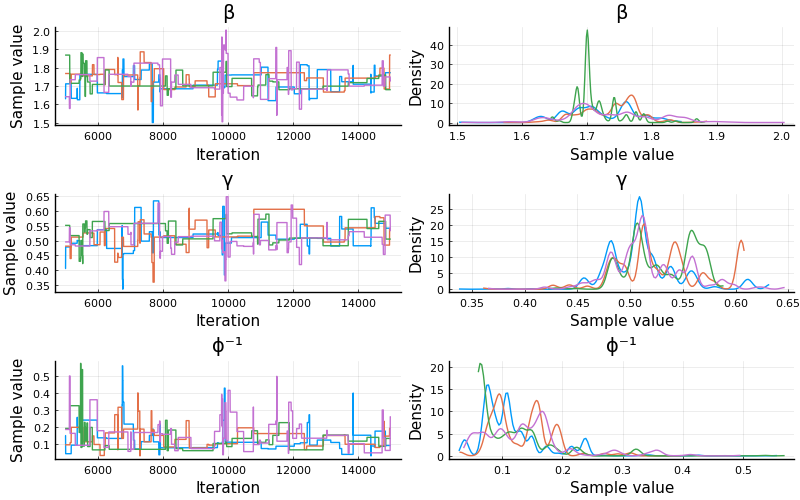
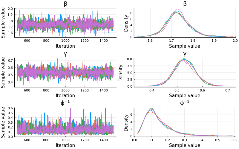
chain = sample(model_conditioned, NUTS(0.8), MCMCThreads(), 1000, 4);
┌ Info: Found initial step size
└   ϵ = 0.8
┌ Info: Found initial step size
└   ϵ = 0.4
┌ Info: Found initial step size
└   ϵ = 0.025
┌ Info: Found initial step size
└   ϵ = 0.05
┌ Warning: The current proposal will be rejected due to numerical error(s).
│   isfinite.((θ, r, ℓπ, ℓκ)) = (true, false, false, false)
└ @ AdvancedHMC ~/.julia/packages/AdvancedHMC/4fByY/src/hamiltonian.jl:49
chain
Chains MCMC chain (1000×15×4 Array{Float64, 3}):

Iterations        = 501:1:1500
Number of chains  = 4
Samples per chain = 1000
Wall duration     = 8.48 seconds
Compute duration  = 33.22 seconds
parameters        = β, γ, ϕ⁻¹
internals         = lp, n_steps, is_accept, acceptance_rate, log_density, hamiltonian_energy, hamiltonian_energy_error, max_hamiltonian_energy_error, tree_depth, numerical_error, step_size, nom_step_size

Summary Statistics
  parameters      mean       std   naive_se      mcse         ess      rhat    ⋯
      Symbol   Float64   Float64    Float64   Float64     Float64   Float64    ⋯

           β    1.7305    0.0532     0.0008    0.0012   2305.3519    1.0006    ⋯
           γ    0.5305    0.0430     0.0007    0.0009   2432.0514    0.9998    ⋯
         ϕ⁻¹    0.1349    0.0727     0.0011    0.0015   2211.5812    0.9994    ⋯
                                                                1 column omitted

Quantiles
  parameters      2.5%     25.0%     50.0%     75.0%     97.5%
      Symbol   Float64   Float64   Float64   Float64   Float64

           β    1.6279    1.6970    1.7281    1.7618    1.8401
           γ    0.4464    0.5024    0.5294    0.5580    0.6172
         ϕ⁻¹    0.0394    0.0843    0.1180    0.1699    0.3165
Muuuch better! Both ESS and Rhat is looking good
plot(chain; size=(800, 500))
# Predict using the results from NUTS.
predictions = predict(model, chain)
Chains MCMC chain (1000×14×4 Array{Float64, 3}):

Iterations        = 1:1:1000
Number of chains  = 4
Samples per chain = 1000
parameters        = in_bed[1], in_bed[2], in_bed[3], in_bed[4], in_bed[5], in_bed[6], in_bed[7], in_bed[8], in_bed[9], in_bed[10], in_bed[11], in_bed[12], in_bed[13], in_bed[14]
internals         =

Summary Statistics
  parameters       mean       std   naive_se      mcse         ess      rhat
      Symbol    Float64   Float64    Float64   Float64     Float64   Float64

   in_bed[1]     3.2840    2.1793     0.0345    0.0327   4055.3023    0.9998
   in_bed[2]    10.7950    5.4560     0.0863    0.0749   3714.2037    1.0005
   in_bed[3]    34.0883   15.7327     0.2488    0.2596   3642.2139    1.0001
   in_bed[4]    93.0002   41.3318     0.6535    0.7048   3577.5458    1.0012
   in_bed[5]   187.5652   79.0050     1.2492    1.2543   3478.9204    1.0010
   in_bed[6]   248.9330   97.2779     1.5381    1.6339   4056.1039    1.0008
   in_bed[7]   234.6240   89.1151     1.4090    1.2074   4022.8396    0.9996
   in_bed[8]   185.4033   71.8807     1.1365    1.0479   3860.3337    0.9997
   in_bed[9]   130.9750   50.4204     0.7972    0.8315   3694.8750    0.9999
  in_bed[10]    88.2115   35.8989     0.5676    0.6532   3401.2244    0.9999
  in_bed[11]    59.4943   25.4118     0.4018    0.4155   3460.7875    0.9997
  in_bed[12]    38.6793   16.7184     0.2643    0.2929   3697.7714    1.0005
  in_bed[13]    24.8678   11.4870     0.1816    0.2081   3578.3080    1.0001
  in_bed[14]    15.9450    8.2237     0.1300    0.1376   3389.6307    0.9996

Quantiles
  parameters      2.5%      25.0%      50.0%      75.0%      97.5%
      Symbol   Float64    Float64    Float64    Float64    Float64

   in_bed[1]    0.0000     2.0000     3.0000     5.0000     8.0000
   in_bed[2]    2.9750     7.0000    10.0000    14.0000    24.0000
   in_bed[3]   11.0000    24.0000    32.0000    42.0000    73.0000
   in_bed[4]   33.0000    65.0000    87.0000   113.0000   190.0000
   in_bed[5]   69.0000   134.0000   177.0000   226.0000   376.0000
   in_bed[6]   95.0000   184.0000   237.0000   299.0000   473.0250
   in_bed[7]   88.0000   175.0000   224.0000   283.0000   440.0250
   in_bed[8]   70.0000   137.0000   176.0000   225.0000   351.0000
   in_bed[9]   49.0000    96.0000   126.0000   159.0000   245.0000
  in_bed[10]   31.9750    64.0000    84.0000   107.0000   170.0000
  in_bed[11]   19.0000    42.0000    57.0000    73.0000   118.0250
  in_bed[12]   13.0000    27.0000    36.0000    48.0000    77.0000
  in_bed[13]    7.0000    17.0000    23.0000    31.0000    51.0000
  in_bed[14]    4.0000    10.0000    15.0000    20.0000    36.0000
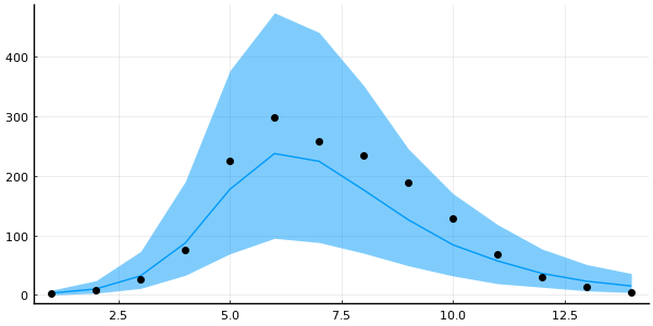
plot_trajectories!(plot(legend=false, size=(600, 300)), predictions; n = 1000, data=data)

plot_trajectory_quantiles!(plot(legend=false, size=(600, 300)), predictions; data=data)
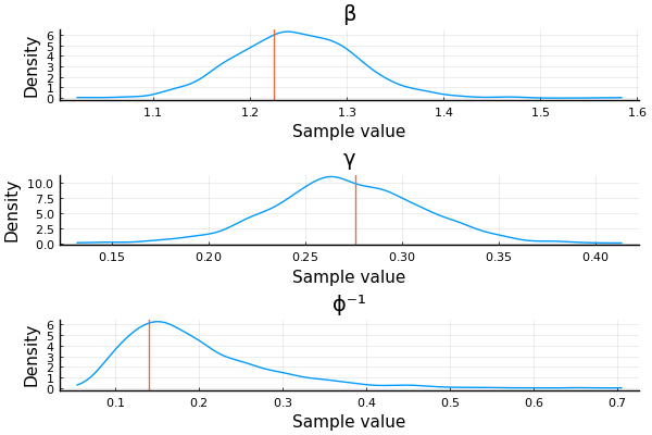
Simulation-based calibration (SBC) Talts et. al. (2018)
- Sample from prior \(\theta_1, \dots, \theta_n \sim p(\theta)\).
- Sample datasets \(\mathcal{D}_i \sim p(\cdot \mid \theta_i)\) for \(i = 1, \dots, n\).
- Obtain (approximate) \(p(\theta \mid \mathcal{D}_i)\) for \(i = 1, \dots, n\).
For large enough (n), the "combination" of the posteriors should recover the prior!
"Combination" here usually means computing some statistic and comparing against what it should be
That's very expensive → in practice we just do this once or twice
# Sample from the conditioned model so we don't get the `in_bed` variables too
using Random  # Just making usre the numbers of somewhat interesting
rng = MersenneTwister(43);
test_values = rand(rng, NamedTuple, model_conditioned)
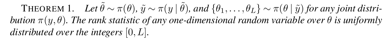
| β | = | 1.2254566808077714 | γ | = | 0.27594266205681933 | ϕ⁻¹ | = | 0.13984179162984164 |
Now we condition on those values and run once to generate data
model_test = model | test_values
Model(
  args = (:problem_wrapper, :prior)
  defaults = ()
  context = ConditionContext((β = 1.2254566808077714, γ = 0.27594266205681933, ϕ⁻¹ = 0.13984179162984164), DynamicPPL.DefaultContext())
)
in_best_test = rand(rng, model_test).in_bed;
Next, inference!
model_test_conditioned = model | (in_bed = in_best_test,)
Model(
  args = (:problem_wrapper, :prior)
  defaults = ()
  context = ConditionContext((in_bed = [1, 9, 11, 45, 159, 136, 270, 123, 463, 376, 231, 148, 99, 162],), DynamicPPL.DefaultContext())
)
# Let's just do a single chain here.
chain_test = sample(model_test_conditioned, NUTS(0.8), 1000);
┌ Info: Found initial step size
└   ϵ = 0.0125

Sampling:   4%|█▊                                       |  ETA: 0:00:05
Sampling:  12%|████▊                                    |  ETA: 0:00:02
Sampling:  25%|██████████▏                              |  ETA: 0:00:01
Sampling:  39%|███████████████▉                         |  ETA: 0:00:01
Sampling:  52%|█████████████████████▍                   |  ETA: 0:00:01
Sampling:  66%|███████████████████████████              |  ETA: 0:00:00
Sampling:  80%|████████████████████████████████▊        |  ETA: 0:00:00
Sampling:  93%|██████████████████████████████████████   |  ETA: 0:00:00
Sampling: 100%|█████████████████████████████████████████| Time: 0:00:01
Did we recover the parameters?
ps = []
for sym in [:β, :γ, :ϕ⁻¹]
    p = density(chain_test[:, [sym], :])
    vline!([test_values[sym]])
    push!(ps, p)
end
plot(ps..., layout=(3, 1), size=(600, 400))
Yay!
Samplers in Turing.jl
- Metropolis-Hastings, emcee, SGLD (AdvancedMH.jl)
- Hamiltonian Monte Carlo, NUTS (AdvancedHMC.jl)
- SMC (AdvancedPS.jl)
- Elliptical Slice Sampling (EllipticalSliceSampling.jl)
- Nested sampling (NestedSamplers.jl)
You can also combine some of these in Turing.jl
using LinearAlgebra: I

@model function linear_regression(X)
    num_params = size(X, 1)
    β ~ MvNormal(ones(num_params))
    σ² ~ InverseGamma(2, 3)
    y ~ MvNormal(vec(β' * X), σ² * I)
end

# Generate some dummy data.
X = randn(2, 1_000); lin_reg = linear_regression(X); true_vals = rand(lin_reg)

# Condition.
lin_reg_conditioned = lin_reg | (y = true_vals.y,);
We can then do Gibbs but sampling \(β\) using ESS and \(\sigma^2\) using HMC
chain_ess_hmc = sample(lin_reg_conditioned, Gibbs(ESS(:β), HMC(1e-3, 16, :σ²)), 1_000)
chain_ess_hmc = sample(lin_reg_conditioned, Gibbs(ESS(:β), HMC(1e-3, 16, :σ²)), 1_000)
Sampling:  10%|████▎                                    |  ETA: 0:00:01
Sampling:  58%|███████████████████████▊                 |  ETA: 0:00:00
Sampling: 100%|█████████████████████████████████████████| Time: 0:00:00
Chains MCMC chain (1000×4×1 Array{Float64, 3}):

Iterations        = 1:1:1000
Number of chains  = 1
Samples per chain = 1000
Wall duration     = 3.39 seconds
Compute duration  = 3.39 seconds
parameters        = β[1], β[2], σ²
internals         = lp

Summary Statistics
  parameters      mean       std   naive_se      mcse        ess      rhat   e ⋯
      Symbol   Float64   Float64    Float64   Float64    Float64   Float64     ⋯

        β[1]   -1.6886    0.1124     0.0036    0.0075   211.1299    1.0006     ⋯
        β[2]   -0.7129    0.0581     0.0018    0.0024   433.8817    1.0015     ⋯
          σ²    1.9929    0.0893     0.0028    0.0113    48.7541    1.0021     ⋯
                                                                1 column omitted

Quantiles
  parameters      2.5%     25.0%     50.0%     75.0%     97.5%
      Symbol   Float64   Float64   Float64   Float64   Float64

        β[1]   -1.7810   -1.7259   -1.6992   -1.6630   -1.6026
        β[2]   -0.7994   -0.7469   -0.7146   -0.6805   -0.6266
          σ²    1.8287    1.9345    1.9893    2.0446    2.1821
Could potentially lead to improvements
NOTE: Usually very difficult to choose sampler parameters in this case
Means one can also mix discrete and continuous
@model function mixture(n)
    cluster ~ filldist(Categorical([0.25, 0.75]), n)
    μ ~ MvNormal([-10.0, 10.0], I)
    x ~ arraydist(Normal.(μ[cluster], 1))
end

model_mixture = mixture(10)
fake_values_mixture = rand(model_mixture)
model_mixture_conditioned = model_mixture | (x = fake_values_mixture.x, )
chain_discrete = sample(
    model_mixture_conditioned, Gibbs(PG(10, :cluster), HMC(1e-3, 16, :μ)), MCMCThreads(), 1_000, 4
)
Sampling (4 threads):  75%|█████████████████████▊       |  ETA: 0:00:00
Sampling (4 threads): 100%|█████████████████████████████| Time: 0:00:00
Chains MCMC chain (1000×13×4 Array{Float64, 3}):

Iterations        = 1:1:1000
Number of chains  = 4
Samples per chain = 1000
Wall duration     = 9.1 seconds
Compute duration  = 35.2 seconds
parameters        = cluster[1], cluster[2], cluster[3], cluster[4], cluster[5], cluster[6], cluster[7], cluster[8], cluster[9], cluster[10], μ[1], μ[2]
internals         = lp

Summary Statistics
   parameters       mean       std   naive_se      mcse         ess      rhat  ⋯
       Symbol    Float64   Float64    Float64   Float64     Float64   Float64  ⋯

   cluster[1]     1.0245    0.1546     0.0024    0.0135     49.1752    1.0586  ⋯
   cluster[2]     1.0517    0.2215     0.0035    0.0244     24.8047    1.1288  ⋯
   cluster[3]     1.1227    0.3282     0.0052    0.0375     18.5621    1.2743  ⋯
   cluster[4]     1.9995    0.0224     0.0004    0.0004   4002.3197    0.9999  ⋯
   cluster[5]     1.9725    0.1636     0.0026    0.0195     25.6370    1.1311  ⋯
   cluster[6]     1.9835    0.1274     0.0020    0.0139     61.8799    1.0723  ⋯
   cluster[7]     1.2712    0.4447     0.0070    0.0532     10.2500    1.9732  ⋯
   cluster[8]     1.0083    0.0905     0.0014    0.0065    128.4567    1.0179  ⋯
   cluster[9]     1.3710    0.4831     0.0076    0.0588     10.7308    1.8081  ⋯
  cluster[10]     2.0000    0.0000     0.0000    0.0000         NaN       NaN  ⋯
         μ[1]   -10.2644    1.1909     0.0188    0.1496      8.0814    8.8935  ⋯
         μ[2]     9.6664    0.8387     0.0133    0.1037      8.4436    3.7077  ⋯
                                                                1 column omitted

Quantiles
   parameters       2.5%      25.0%      50.0%     75.0%     97.5%
       Symbol    Float64    Float64    Float64   Float64   Float64

   cluster[1]     1.0000     1.0000     1.0000    1.0000    1.0000
   cluster[2]     1.0000     1.0000     1.0000    1.0000    2.0000
   cluster[3]     1.0000     1.0000     1.0000    1.0000    2.0000
   cluster[4]     2.0000     2.0000     2.0000    2.0000    2.0000
   cluster[5]     1.0000     2.0000     2.0000    2.0000    2.0000
   cluster[6]     2.0000     2.0000     2.0000    2.0000    2.0000
   cluster[7]     1.0000     1.0000     1.0000    2.0000    2.0000
   cluster[8]     1.0000     1.0000     1.0000    1.0000    1.0000
   cluster[9]     1.0000     1.0000     1.0000    2.0000    2.0000
  cluster[10]     2.0000     2.0000     2.0000    2.0000    2.0000
         μ[1]   -11.8037   -11.3141   -10.4745   -9.3795   -8.2947
         μ[2]     8.4038     8.9560     9.6131   10.4825   11.0633
ps = []
for (i, realizations) in enumerate(eachcol(Array(group(chain_discrete, :cluster))))
    p = density(realizations, legend=false, ticks=false); vline!(p, [fake_values_mixture.cluster[i]])
    push!(ps, p)
end
plot(ps..., layout=(length(ps) ÷ 2, 2), size=(600, 40 * length(ps)))
Again, this is difficult to get to work properly on non-trivial examples
But it is possible
Other utilities for Turing.jl
- TuringGLM.jl: GLMs using the formula-syntax from R but using Turing.jl under the hood
- TuringBenchmarking.jl: useful for benchmarking Turing.jl models
- TuringCallbacks.jl: on-the-fly visualizations using
tensorboard

Downsides of using Turing.jl
- Don't do any depedency-extraction of the model ⟹ can't do things like automatic marginalization
- But it's not impossible; just a matter of development effort
- Ongoing work in
TuringLangto make a BUGS compatible model "compiler" / parser (in colab with Andrew Thomas & others)
- NUTS performance is at the mercy of AD in Julia
- You can put anything in your model, but whether you should is a another matter
Benchmarking
using SciMLSensitivity
using BenchmarkTools
using TuringBenchmarking
using ReverseDiff, Zygote
suite = TuringBenchmarking.make_turing_suite(
    model_conditioned;
    adbackends=[
        TuringBenchmarking.ForwardDiffAD{40,true}(),
        TuringBenchmarking.ReverseDiffAD{false}(),
        TuringBenchmarking.ZygoteAD()
    ]
);
run(suite)
2-element BenchmarkTools.BenchmarkGroup:
  tags: []
  "linked" => 4-element BenchmarkTools.BenchmarkGroup:
	  tags: []
	  "Turing.Essential.ReverseDiffAD{false}()" => Trial(368.161 μs)
	  "evaluation" => Trial(28.270 μs)
	  "Turing.Essential.ForwardDiffAD{40, true}()" => Trial(122.734 μs)
	  "Turing.Essential.ZygoteAD()" => Trial(3.121 ms)
  "not_linked" => 4-element BenchmarkTools.BenchmarkGroup:
	  tags: []
	  "Turing.Essential.ReverseDiffAD{false}()" => Trial(454.382 μs)
	  "evaluation" => Trial(27.078 μs)
	  "Turing.Essential.ForwardDiffAD{40, true}()" => Trial(151.882 μs)
	  "Turing.Essential.ZygoteAD()" => Trial(2.885 ms)
More data
Let's add some more timesteps to make it a more interesting
How about 10 000?
# NOTE: We now use 10 000 days instead of just 14.
model_fake = epidemic_model(SIRProblem(N; tspan=(0, 10_000)), prior_improved);
From this we'll generate some fake data
res = rand(model_fake)
model_fake_conditioned = model_fake | (in_bed = res.in_bed,);
model_fake_conditioned().infected
10000-element Vector{Float64}:
   2.7975983440413223
   7.748418187214023
  20.88236766334096
  52.45691560357974
 112.4569199051879
 183.12340579979855
 215.7666283305088
 196.72101213557013
 153.56623546042505
 110.06252620822383
  75.3051039014327
  50.188689698069695
  32.953929054350986
   ⋮
  -4.200904016575503e-16
  -3.884354912599255e-16
  -3.5677074858373597e-16
  -3.2509617362904785e-16
  -2.934117663958071e-16
  -2.6171752688401963e-16
  -2.300134550937096e-16
  -1.9829955102488296e-16
  -1.6657581467747957e-16
  -1.3484224605157163e-16
  -1.0309884514710501e-16
  -7.134561196412778e-17
And run some benchmarks!
suite = TuringBenchmarking.make_turing_suite(
    model_fake_conditioned;
    adbackends=[
        TuringBenchmarking.ForwardDiffAD{40,true}(),
        TuringBenchmarking.ReverseDiffAD{false}(),
        TuringBenchmarking.ZygoteAD()
    ]
);
run(suite)
2-element BenchmarkTools.BenchmarkGroup:
  tags: []
  "linked" => 4-element BenchmarkTools.BenchmarkGroup:
	  tags: []
	  "Turing.Essential.ReverseDiffAD{false}()" => Trial(42.524 ms)
	  "evaluation" => Trial(2.020 ms)
	  "Turing.Essential.ForwardDiffAD{40, true}()" => Trial(3.687 ms)
	  "Turing.Essential.ZygoteAD()" => Trial(29.392 ms)
  "not_linked" => 4-element BenchmarkTools.BenchmarkGroup:
	  tags: []
	  "Turing.Essential.ReverseDiffAD{false}()" => Trial(40.269 ms)
	  "evaluation" => Trial(2.035 ms)
	  "Turing.Essential.ForwardDiffAD{40, true}()" => Trial(3.826 ms)
	  "Turing.Essential.ZygoteAD()" => Trial(32.606 ms)
What if we use a different sensealg in solve?
@model function epidemic_model(
    problem_wrapper::AbstractEpidemicProblem,
    prior;
    sensealg=ForwardDiffSensitivity()  # NOTE: This will be passed to `solve`.
)
    # And use `@submodel` to embed the `prior` in our model.
    @submodel p = prior(problem_wrapper)

    ϕ⁻¹ ~ Exponential(1/5)
    ϕ = inv(ϕ⁻¹)

    problem_new = remake(problem_wrapper.problem, p=p)    # Replace parameters `p`.
    # NOTE: Allowed to use a different `sensealg`
    sol = solve(problem_new; saveat=1, sensealg=sensealg) # Solve!

    # Return early if integration failed.
    if !issuccess(sol)
        Turing.@addlogprob! -Inf  # Causes automatic rejection.
        return nothing
    end

    # Extract the `infected`.
    sol_for_observed = infected(problem_wrapper, sol)[2:end]

    # `arraydist` is faster for larger dimensional problems,
    # and it does not require explicit allocation of the vector.
    in_bed ~ arraydist(NegativeBinomial2.(sol_for_observed .+ 1e-5, ϕ))

    β, γ = p[1:2]
    return (R0 = β / γ, recovery_time = 1 / γ, infected = sol_for_observed)
end
epidemic_model (generic function with 3 methods)
model_fake = epidemic_model(
    SIRProblem(N; tspan=(0, 10_000)),
    prior_improved;
    sensealg=ForwardSensitivity()  # NOTE: `ForwardSensitivity` is differnt from `ForwardDiffSensitivity`
);
model_fake_conditioned = model_fake | (in_bed = res.in_bed,);
# NOTE: AFAIK `ForwardSensitivity` has no effect when used with `ForwardDiff.jl`.
suite = TuringBenchmarking.make_turing_suite(
    model_fake_conditioned;
    adbackends=[
        TuringBenchmarking.ReverseDiffAD{false}(),
        TuringBenchmarking.ZygoteAD()
    ]
);
run(suite)
2-element BenchmarkTools.BenchmarkGroup:
  tags: []
  "linked" => 3-element BenchmarkTools.BenchmarkGroup:
	  tags: []
	  "Turing.Essential.ReverseDiffAD{false}()" => Trial(21.775 ms)
	  "evaluation" => Trial(2.104 ms)
	  "Turing.Essential.ZygoteAD()" => Trial(10.506 ms)
  "not_linked" => 3-element BenchmarkTools.BenchmarkGroup:
	  tags: []
	  "Turing.Essential.ReverseDiffAD{false}()" => Trial(23.455 ms)
	  "evaluation" => Trial(1.889 ms)
	  "Turing.Essential.ZygoteAD()" => Trial(11.741 ms)
Okay, so it's faster but ForwardDiff.jl still wins
(which is not surprising on such a low-dimensional problem)
Case: spatio-temporal COVID modeling in UK

Main model looked like this
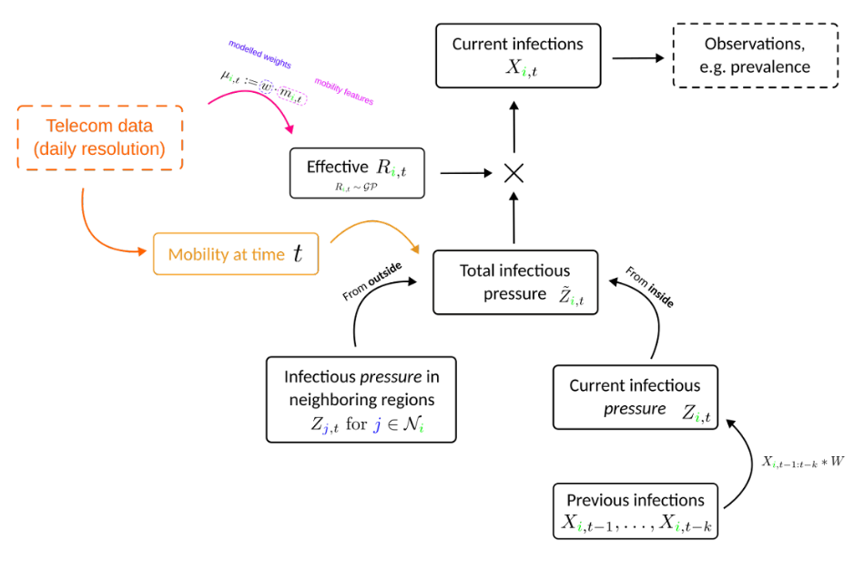
Roughly 50 000 parameters
Output, for different approaches, looked like this
# GP-model for R-value.
@submodel R = SpatioTemporalGP(K_spatial, K_local, K_time, T; σ_spatial, σ_local, ρ_spatial, ρ_time)

# Latent infections.
@submodel X = RegionalFlux(F_id, F_in, F_out, W, R, X_cond, T; days_per_step, σ_ξ)

# Likelihood.
@submodel C = NegBinomialWeeklyAdjustedTesting(C, X, D, num_cond, T)
with
@model function SpatioTemporalGP(
    K_spatial, K_local, K_time,
    ::Type{T} = Float64;
) where {T}
    num_steps = size(K_time, 1)
    num_regions = size(K_spatial, 1)

    # Length scales
    ρ_spatial ~ 𝒩₊(T(0), T(5))
    ρ_time ~ 𝒩₊(T(0), T(5))

    # Scales
    σ_spatial ~ 𝒩₊(T(0), T(0.5))
    σ_local ~ 𝒩₊(T(0), T(0.5))

    # GP
    E_vec ~ MvNormal(num_regions * num_steps, one(T))
    E = reshape(E_vec, (num_regions, num_steps))

    # Get cholesky decomps using precomputed kernel matrices
    L_space = spatial_L(K_spatial, K_local, σ_spatial, σ_local, ρ_spatial)
    U_time = time_U(K_time, ρ_time)

    # Obtain realization of log-R.
    f = L_space * E * U_time

    # Compute R.
    R = exp.(f)
    return R
end
Julia: The Good, the Bad, and the Ugly
An honest take from a little 27-year old Norwegian boy
The Good
- Speed
- Composability (thank you multiple dispatch)
- No need to tie yourself to an underlying computational framework
- Interactive
- Transparency
- Very easy to call into other languages
Speed
I think you got this already…
Composability
We've seen some of that
Defining infected(problem_wrapper, u) allowed us to abstract away how to extract the compartment of interest
Transparency
For starters, almost all the code you'll end up using is pure Julia
Hence, you can always look at the code
You can find the implementation by using @which
# Without arguments
@which sum
Base
# With arguments
@which sum([1.0])
sum(a::AbstractArray; dims, kw...) in Base at reducedim.jl:994
And yeah, you can even look into the macros
@macroexpand @model f() = x ~ Normal()
quote
    function f(__model__::DynamicPPL.Model, __varinfo__::DynamicPPL.AbstractVarInfo, __context__::AbstractPPL.AbstractContext; )
        #= In[113]:1 =#
        begin
            var"##dist#1413" = Normal()
            var"##vn#1410" = (DynamicPPL.resolve_varnames)((AbstractPPL.VarName){:x}(), var"##dist#1413")
            var"##isassumption#1411" = begin
                    if (DynamicPPL.contextual_isassumption)(__context__, var"##vn#1410")
                        if !((DynamicPPL.inargnames)(var"##vn#1410", __model__)) || (DynamicPPL.inmissings)(var"##vn#1410", __model__)
                            true
                        else
                            x === missing
                        end
                    else
                        false
                    end
                end
            begin
                #= /home/tor/.julia/packages/DynamicPPL/WBmMU/src/compiler.jl:539 =#
                var"##retval#1415" = if var"##isassumption#1411"
                        begin
                            (var"##value#1414", __varinfo__) = (DynamicPPL.tilde_assume!!)(__context__, (DynamicPPL.unwrap_right_vn)((DynamicPPL.check_tilde_rhs)(var"##dist#1413"), var"##vn#1410")..., __varinfo__)
                            x = var"##value#1414"
                            var"##value#1414"
                        end
                    else
                        if !((DynamicPPL.inargnames)(var"##vn#1410", __model__))
                            x = (DynamicPPL.getvalue_nested)(__context__, var"##vn#1410")
                        end
                        (var"##value#1412", __varinfo__) = (DynamicPPL.tilde_observe!!)(__context__, (DynamicPPL.check_tilde_rhs)(var"##dist#1413"), x, var"##vn#1410", __varinfo__)
                        var"##value#1412"
                    end
                #= /home/tor/.julia/packages/DynamicPPL/WBmMU/src/compiler.jl:540 =#
                return (var"##retval#1415", __varinfo__)
            end
        end
    end
    begin
        $(Expr(:meta, :doc))
        function f(; )
            #= In[113]:1 =#
            return (DynamicPPL.Model)(f, NamedTuple(), NamedTuple())
        end
    end
end
I told you didn't want to see that.
Can make it a bit cleaner by removing linenums:
@macroexpand(@model f() = x ~ Normal()) |> Base.remove_linenums!
quote
    function f(__model__::DynamicPPL.Model, __varinfo__::DynamicPPL.AbstractVarInfo, __context__::AbstractPPL.AbstractContext; )
        begin
            var"##dist#1419" = Normal()
            var"##vn#1416" = (DynamicPPL.resolve_varnames)((AbstractPPL.VarName){:x}(), var"##dist#1419")
            var"##isassumption#1417" = begin
                    if (DynamicPPL.contextual_isassumption)(__context__, var"##vn#1416")
                        if !((DynamicPPL.inargnames)(var"##vn#1416", __model__)) || (DynamicPPL.inmissings)(var"##vn#1416", __model__)
                            true
                        else
                            x === missing
                        end
                    else
                        false
                    end
                end
            begin
                var"##retval#1421" = if var"##isassumption#1417"
                        begin
                            (var"##value#1420", __varinfo__) = (DynamicPPL.tilde_assume!!)(__context__, (DynamicPPL.unwrap_right_vn)((DynamicPPL.check_tilde_rhs)(var"##dist#1419"), var"##vn#1416")..., __varinfo__)
                            x = var"##value#1420"
                            var"##value#1420"
                        end
                    else
                        if !((DynamicPPL.inargnames)(var"##vn#1416", __model__))
                            x = (DynamicPPL.getvalue_nested)(__context__, var"##vn#1416")
                        end
                        (var"##value#1418", __varinfo__) = (DynamicPPL.tilde_observe!!)(__context__, (DynamicPPL.check_tilde_rhs)(var"##dist#1419"), x, var"##vn#1416", __varinfo__)
                        var"##value#1418"
                    end
                return (var"##retval#1421", __varinfo__)
            end
        end
    end
    begin
        $(Expr(:meta, :doc))
        function f(; )
            return (DynamicPPL.Model)(f, NamedTuple(), NamedTuple())
        end
    end
end
f(x) = 2x
f (generic function with 1 method)
You can inspect the type-inferred and lowered code
@code_typed f(1)
CodeInfo(
1 ─ %1 = Base.mul_int(2, x)::Int64
└──      return %1
) => Int64
You can inspect the LLVM code
@code_llvm f(1)
;  @ In[115]:1 within `f`
define i64 @julia_f_52767(i64 signext %0) #0 {
top:
; ┌ @ int.jl:88 within `*`
   %1 = shl i64 %0, 1
; └
  ret i64 %1
}
And even the resulting machine code
@code_native f(1)
	.text
	.file	"f"
	.globl	julia_f_52804                   # -- Begin function julia_f_52804
	.p2align	4, 0x90
	.type	julia_f_52804,@function
julia_f_52804:                          # @julia_f_52804
; ┌ @ In[115]:1 within `f`
	.cfi_startproc
# %bb.0:                                # %top
; │┌ @ int.jl:88 within `*`
	leaq	(%rdi,%rdi), %rax
; │└
	retq
.Lfunc_end0:
	.size	julia_f_52804, .Lfunc_end0-julia_f_52804
	.cfi_endproc
; └
                                        # -- End function
	.section	".note.GNU-stack","",@progbits
It really just depends on which level of "I hate my life" you're currently at
Calling into other languages
- C and Fortran comes built-in stdlib
- RCall.jl: call into
R - PyCall.jl: call into
python - Etc.
When working with Array, etc. memory is usually shared ⟹ fairly low overhead
C and Fortran
# Define the Julia function
function mycompare(a, b)::Cint
    println("mycompare($a, $b)")  # NOTE: Let's look at the comparisons made.
    return (a < b) ? -1 : ((a > b) ? +1 : 0)
end

# Get the corresponding C function pointer.
mycompare_c = @cfunction(mycompare, Cint, (Ref{Cdouble}, Ref{Cdouble}))

# Array to sort.
arr = [1.3, -2.7, 4.4, 3.1];

# Call in-place quicksort.
ccall(:qsort, Cvoid, (Ptr{Cdouble}, Csize_t, Csize_t, Ptr{Cvoid}),
      arr, length(arr), sizeof(eltype(arr)), mycompare_c)
mycompare(1.3, -2.7)
mycompare(4.4, 3.1)
mycompare(-2.7, 3.1)
mycompare(1.3, 3.1)
# All sorted!
arr
4-element Vector{Float64}:
 -2.7
  1.3
  3.1
  4.4
The Bad
Sometimes
- your code might just slow down without a seemingly good reason,
- someone did bad, and Julia can't tell which method to call, or
- someone forces the Julia compiler to compile insane amounts of code
"Why is my code suddenly slow?"
One word: type-instability
Sometimes the Julia compiler can't quite infer what types fully
Result: python-like performance (for those particular function calls)
# NOTE: this is NOT `const`, and so it could become some other type
# at any given point without `my_func` knowing about it!
global_variable = 1
my_func_unstable(x) = global_variable * x
my_func_unstable (generic function with 1 method)
@btime my_func_unstable(2.0);
30.668 ns (2 allocations: 32 bytes)
Luckily there are tools for inspecting this
@code_warntype my_func_unstable(2.0)
MethodInstance for my_func_unstable(::Float64)
  from my_func_unstable(x) in Main at In[121]:4
Arguments
  #self#::Core.Const(my_func_unstable)
  x::Float64
Body::Any
1 ─ %1 = (Main.global_variable * x)::Any
└──      return %1
See that Any there? 'tis a big no-no!
Once discovered, it can be fixed
const constant_global_variable = 1
my_func_fixed(x) = constant_global_variable * x
@code_warntype my_func_fixed(2.0)
MethodInstance for my_func_fixed(::Float64)
  from my_func_fixed(x) in Main at In[124]:2
Arguments
  #self#::Core.Const(my_func_fixed)
  x::Float64
Body::Float64
1 ─ %1 = (Main.constant_global_variable * x)::Float64
└──      return %1
So long Python performance!
@btime my_func_fixed(2.0);
1.696 ns (0 allocations: 0 bytes)
But this is not always so easy to discover (though this is generally rare)
# HACK: Here we explicitly tell Julia what type `my_func_unstable`
# returns. This is _very_ rarely a good idea because it just hides
# the underlying problem from `@code_warntype`!
my_func_forced(x) = my_func_unstable(x)::typeof(x)
@code_warntype my_func_forced(2.0)
MethodInstance for my_func_forced(::Float64)
  from my_func_forced(x) in Main at In[126]:4
Arguments
  #self#::Core.Const(my_func_forced)
  x::Float64
Body::Float64
1 ─ %1 = Main.my_func_unstable(x)::Any
│   %2 = Main.typeof(x)::Core.Const(Float64)
│   %3 = Core.typeassert(%1, %2)::Float64
└──      return %3
We can still see the Any in there, but on a first glance it looks like my_func_forced is type-stable
There are more natural cases where this might occur, e.g. unfortunate closures deep in your callstack
To discovery these there are a couple of more advanced tools:
- Cthulhu.jl: Allows you to step through your code like a debugger and perform
@code_warntype - JET.jl: Experimental package which attempts to automate the process
And even simpler: profile using ProfileView.jl and look for code-paths that should be fast but take up a lot of the runtime
using ProfileView
@profview foreach(_ -> my_func_unstable(2.0), 1_000_000)

Note that there's no sign of multiplication here
But most of the runtime is the ./reflection.jl at the top there
That's Julia looking up the type at runtime
Method ambiguity
ambiguous_function(x, y::Int) = y
ambiguous_function(x::Int, y) = x

# NOTE: Here we have `ambiguous_function(x::Int, y::Int)`
# Which one should we hit?!
ambiguous_function(1, 2)
MethodError: ambiguous_function(::Int64, ::Int64) is ambiguous. Candidates:
  ambiguous_function(x, y::Int64) in Main at In[128]:1
  ambiguous_function(x::Int64, y) in Main at In[128]:2
Possible fix, define
  ambiguous_function(::Int64, ::Int64)

Stacktrace:
 [1] top-level scope
   @ In[128]:6
But here Julia warns us, and so we can fix this by just doing as it says: define ambiguous_function(::Int64, ::Int64)
ambiguous_function(::Int64, ::Int64) = "neato"
ambiguous_function(1, 2)
"neato"
Long compilation times
In Julia, for better or worse, we can generate code
Problem: it can be lots of code of we really want to
Result: first execution can be slow
Time to first plot (TTFP) is Julia's worst enemy
But things are always improving

Another example: mis-use of @generated
# NOTE: `@generated` only has access to static information, e.g. types of arguments.
# Here I'm using the special type `Val` to make a number `N` static.
@generated function unrolled_addition(::Val{N}) where {N}
    expr = Expr(:block)
    push!(expr.args, :(x = 0))
    for i = 1:N
        push!(expr.args, :(x += $(3.14 * i)))
    end

    return expr
end
unrolled_addition (generic function with 1 method)
When I call this with some Val(N), Julia will execute this at compile-time!
# NOTE: At runtime, it then just returns the result immediately
@code_typed unrolled_addition(Val(10))
CodeInfo(
1 ─     return 172.70000000000002
) => Float64
But if I just change the value 10 to 11, it's a completely different type!
So Julia has to compile unrolled_addition from scratch
@time @eval unrolled_addition(Val(11));
0.010027 seconds (11.61 k allocations: 654.885 KiB, 8.32% compilation time)
Or a bit crazier
@time @eval unrolled_addition(Val(10_001));
0.429549 seconds (1.19 M allocations: 48.946 MiB, 99.94% compilation time)
Here it took ~0.4s, of which 99.95% was compilation time
I think you get the idea
But boy is it fast to run!
@btime unrolled_addition(Val(10_001));
1.637 ns (0 allocations: 0 bytes)
function not_unrolled_addition(N)
    x = 0
    for i = 1:N
        x += 3.14 * i
    end

    return x
end
not_unrolled_addition (generic function with 1 method)
@btime not_unrolled_addition(10_001);
11.138 μs (0 allocations: 0 bytes)
Funny side-note: at first I did the following
@generated function unrolled_addition_old(::Val{N}) where {N}
    expr = Expr(:block)
    push!(expr.args, :(x = 0))
    for i = 1:N
        push!(expr.args, :(x += $i))  # NOTE: No 3.14!
    end
    return expr
end
function not_unrolled_addition_old(N)
    x = 0
    for i = 1:N
        x += i  # NOTE: No 3.14!
    end
    return x
end
not_unrolled_addition_old (generic function with 1 method)
@btime unrolled_addition_old(Val(10_001));
@btime not_unrolled_addition_old(10_001);
1.538 ns (0 allocations: 0 bytes)
3.495 ns (0 allocations: 0 bytes)
LLVM probably recognized the pattern of not_unrolled_addition_old and unrolls it for us
Let's check!
# NOTE: The one LLVM failed to unroll
@code_llvm not_unrolled_addition(10_001)
;  @ In[135]:1 within `not_unrolled_addition`
define { {}*, i8 } @julia_not_unrolled_addition_53856([8 x i8]* noalias nocapture align 8 dereferenceable(8) %0, i64 signext %1) #0 {
top:
;  @ In[135]:3 within `not_unrolled_addition`
; ┌ @ range.jl:5 within `Colon`
; │┌ @ range.jl:393 within `UnitRange`
; ││┌ @ range.jl:400 within `unitrange_last`
     %.inv = icmp sgt i64 %1, 0
     %. = select i1 %.inv, i64 %1, i64 0
; └└└
  br i1 %.inv, label %L18.preheader, label %union_move16

L18.preheader:                                    ; preds = %top
;  @ In[135]:5 within `not_unrolled_addition`
; ┌ @ range.jl:883 within `iterate`
; │┌ @ promotion.jl:477 within `==`
    %.not30 = icmp eq i64 %., 1
; └└
  br i1 %.not30, label %union_move, label %L51

L51:                                              ; preds = %L51, %L18.preheader
  %value_phi1032 = phi double [ %value_phi10, %L51 ], [ 3.140000e+00, %L18.preheader ]
  %value_phi431 = phi i64 [ %2, %L51 ], [ 1, %L18.preheader ]
; ┌ @ range.jl:883 within `iterate`
   %2 = add i64 %value_phi431, 1
; └
;  @ In[135]:4 within `not_unrolled_addition`
; ┌ @ promotion.jl:389 within `*`
; │┌ @ promotion.jl:359 within `promote`
; ││┌ @ promotion.jl:336 within `_promote`
; │││┌ @ number.jl:7 within `convert`
; ││││┌ @ float.jl:146 within `Float64`
       %3 = sitofp i64 %2 to double
; │└└└└
; │ @ promotion.jl:389 within `*` @ float.jl:385
   %4 = fmul double %3, 3.140000e+00
; └
;  @ In[135] within `not_unrolled_addition`
  %value_phi10 = fadd double %value_phi1032, %4
;  @ In[135]:5 within `not_unrolled_addition`
; ┌ @ range.jl:883 within `iterate`
; │┌ @ promotion.jl:477 within `==`
    %.not = icmp eq i64 %2, %.
; └└
  br i1 %.not, label %L18.union_move_crit_edge, label %L51

post_union_move:                                  ; preds = %union_move16, %union_move
  %tindex_phi1429 = phi i8 [ 2, %union_move16 ], [ 1, %union_move ]
;  @ In[135]:7 within `not_unrolled_addition`
  %5 = insertvalue { {}*, i8 } { {}* null, i8 undef }, i8 %tindex_phi1429, 1
  ret { {}*, i8 } %5

L18.union_move_crit_edge:                         ; preds = %L51
;  @ In[135]:5 within `not_unrolled_addition`
  %phi.cast = bitcast double %value_phi10 to i64
  br label %union_move

union_move:                                       ; preds = %L18.union_move_crit_edge, %L18.preheader
  %value_phi10.lcssa = phi i64 [ %phi.cast, %L18.union_move_crit_edge ], [ 4614253070214989087, %L18.preheader ]
;  @ In[135]:7 within `not_unrolled_addition`
  %6 = bitcast [8 x i8]* %0 to i64*
  store i64 %value_phi10.lcssa, i64* %6, align 8
  br label %post_union_move

union_move16:                                     ; preds = %top
  %7 = bitcast [8 x i8]* %0 to i64*
  store i64 0, i64* %7, align 8
  br label %post_union_move
}
# NOTE: The one LLVM seems to have unrolled.
@code_llvm not_unrolled_addition_old(10_001)
;  @ In[137]:9 within `not_unrolled_addition_old`
define i64 @julia_not_unrolled_addition_old_53858(i64 signext %0) #0 {
top:
;  @ In[137]:11 within `not_unrolled_addition_old`
; ┌ @ range.jl:5 within `Colon`
; │┌ @ range.jl:393 within `UnitRange`
; ││┌ @ range.jl:400 within `unitrange_last`
     %.inv = icmp sgt i64 %0, 0
     %. = select i1 %.inv, i64 %0, i64 0
; └└└
  br i1 %.inv, label %L18.preheader, label %L35

L18.preheader:                                    ; preds = %top
;  @ In[137]:13 within `not_unrolled_addition_old`
  %1 = shl nuw i64 %., 1
  %2 = add nsw i64 %., -1
  %3 = zext i64 %2 to i65
  %4 = add nsw i64 %., -2
  %5 = zext i64 %4 to i65
  %6 = mul i65 %3, %5
  %7 = lshr i65 %6, 1
  %8 = trunc i65 %7 to i64
  %9 = add i64 %1, %8
  %10 = add i64 %9, -1
;  @ In[137]:14 within `not_unrolled_addition_old`
  br label %L35

L35:                                              ; preds = %L18.preheader, %top
  %value_phi10 = phi i64 [ 0, %top ], [ %10, %L18.preheader ]
  ret i64 %value_phi10
}
The Ugly
Reverse-mode automatic differentiation
ForwardDiff.jl is a pure joy, but slows down as dimensionality grows
Then one should reach for ReverseDiff.jl or Zygote.jl
Most of the time it works really well, but sometimes you hit a real sharp edge
And sharp edges cut; they cut deep
Like "16X slower when the function is implemented more efficiently"-deep

If you want to see a man in pain, you can find the full issue here
On the flip-side, once addressed (a type-instability), it's 3X faster than before
Overall
Julia is pretty darn awesome
Easy to get going, and you can always make it faster by just optimizing your Julia code
No need to drop down to C++
Buuuut it can't beat Python at deep learning
Otherwise, it's worth a try
Godspeed to you
Fin.